Neural Jastrow

In this tutorial, we use neural networks as generalized Jastrow factors to study the Heisenberg J1-J2 model.

Reference:

Y. Normura, et al., Restricted Boltzmann machine learning for solving strongly correlated quantum systems, Phys. Rev. B 96, 205152 (2017).

Y. Normura and M. Imada, Dirac-Type Nodal Spin Liquid Revealed by Refined Quantum Many-Body Solver Using Neural-Network Wave Function, Correlation Ratio, and Level Spectroscopy, Phys. Rev. X 11, 031034 (2021).

import numpy as np
import matplotlib.pyplot as plt
import jax.numpy as jnp
import equinox as eqx
import quantax as qtx
from IPython.display import clear_output

lattice = qtx.sites.Square(4, Nparticles=(8, 8))
N = lattice.Nsites

The Hamiltonian is

\[ H = J_1 \sum_{\braket{ij}} \mathbf{\sigma}_i \cdot \mathbf{\sigma}_j + J_2 \sum_{\braket{\braket{ij}}} \mathbf{\sigma}_i \cdot \mathbf{\sigma}_j, \]

where \(\braket{ij}\) and \(\braket{\braket{ij}}\) represent nearest and next-nearest neighbors, respectively.

from quantax.symmetry import Identity, TransND, C4v, SpinInverse

H = qtx.operator.Heisenberg(J=[1, 0.5], n_neighbor=[1, 2])

full_symm = TransND() @ C4v() @ SpinInverse()
E, psi = H.diagonalize(symm=full_symm)
exact_energy = E[0]
exact_state = qtx.state.DenseState(psi, full_symm)
print("Exact ground state energy:", exact_energy)

Exact ground state energy: -33.83169340557937

/home/aochen/quantax_env/lib/python3.12/site-packages/quantax/symmetry/symmetry.py:288: GeneralBasisWarning: using non-commuting symmetries can lead to unwanted behaviour of general basis, make sure that quantum numbers are invariant under non-commuting symmetries!
  basis = spin_basis_general(

Gutzwiller-projected fermionic wavefunction

The Hamiltonian in spin degrees of freedom can be mapped to fermion ones by

\[\begin{split} S^\alpha = \frac{1}{2} (c_\uparrow^\dagger, c_\downarrow^\dagger) \sigma^\alpha \begin{pmatrix} c_\uparrow \\ c_\downarrow \end{pmatrix}, \end{split}\]

where \(\alpha = x,y,z\) and \(\sigma^\alpha\) are Pauli matrices. Quantax utilizes this relation internally such that the mean-field state can be optimized in spin systems.

A fermionic wavefunction \(\ket{\psi_0}\) contains redundancy of zero occupancy and double occupancy when it is used for spin systems. Therefore, one needs a Gutzwiller projection to obtain

\[ \ket{\psi_G} = \hat P_G \ket{\psi_0}, \]

where \(\hat P_G = \prod_i (n_{i\uparrow} - n_{i\downarrow})^2\) projects the state to spin degrees of freedom. In variational Monte Carlo, this is done by sampling suitable sectors instead of modifying the mean-field state.

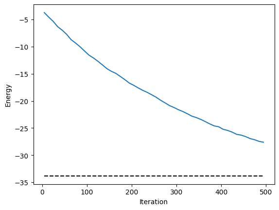
Here we show how to optimize the Gutzwiller-projected fermionic mean-field wavefunction. GeneralPfState is a subclass of Variational, so one can train it directly with SR.

state = qtx.state.GeneralPfState(max_parallel=32768)
sampler = qtx.sampler.SpinExchange(state, 1024, n_neighbor=[1, 2])
optimizer = qtx.optimizer.SR(state, H)

energy = qtx.utils.DataTracer()
VarE = qtx.utils.DataTracer()

for i in range(500):
    samples = sampler.sweep()
    step = optimizer.get_step(samples)
    state.update(step * 1e-3)

    energy.append(optimizer.energy)
    VarE.append(optimizer.VarE)

energy.plot(batch=10, baseline=exact_energy)
plt.xlabel("Iteration")
plt.ylabel("Energy")
plt.show()
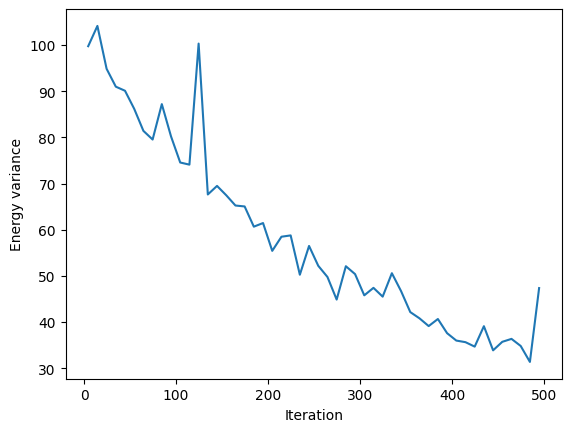
VarE.plot(batch=10)
plt.xlabel("Iteration")
plt.ylabel("Energy variance")
plt.show()

Neural Jastrow factor

The neural Jastrow factor modifies an existing wavefunction by utilizing a neural network. The new wavefunction is given by

\[ \psi(s) = J(s) \psi_G(s), \]

where \(J(s)\) is the neural Jastrow factor, and \(\psi_G(s)\) is the original Gutzwiller-projected fermionic wavefunction.

We can take the pre-trained Pfaffian state as a good initialization.

pf_model = state.model

We still utilize ResConv as the neural network. trans_symm=Identity() means network output is not summed in the last layer, so the output is a matrix \(\mathbf{J}(s)\). Then we define NeuralJastrow with trans_symm=TransND(), which means the output is

\[ \psi(s) = \sum_i^{L_x} \sum_j^{L_y} \mathbf{J}_{ij}(s) \psi_G(T_{ij}s), \]

where \(T_{ij}s\) is a translation of the original input \(s\). One can view this formula as a translation symmetrized form of \(\psi(s) = J(s) \psi_G(s)\).

net = qtx.model.ResConv(nblocks=2, channels=8, kernel_size=3, trans_symm=Identity())
model = qtx.model.NeuralJastrow(net, pf_model, trans_symm=TransND())

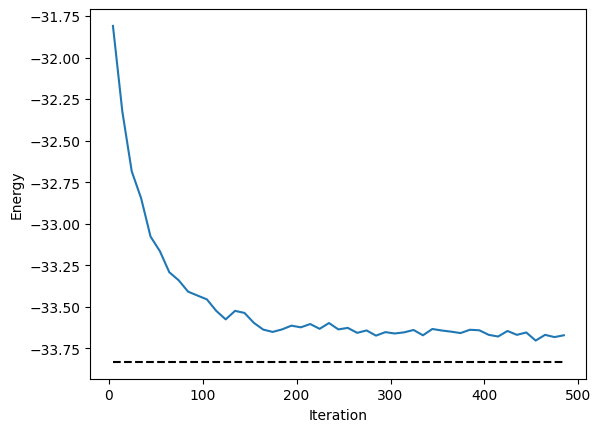
Then one can perform the usual SR optimization on this wavefunction.

state = qtx.state.Variational(model, max_parallel=16384)

sampler = qtx.sampler.SpinExchange(state, 1024, n_neighbor=[1, 2])
optimizer = qtx.optimizer.SR(state, H)

energy = qtx.utils.DataTracer()
VarE = qtx.utils.DataTracer()

for i in range(500):
    samples = sampler.sweep()
    step = optimizer.get_step(samples)
    state.update(step * 2e-3)

    energy.append(optimizer.energy)
    VarE.append(optimizer.VarE)

    if i % 10 == 0:
        clear_output()
        energy.plot(batch=10, baseline=exact_energy)
        plt.xlabel("Iteration")
        plt.ylabel("Energy")
        plt.show()
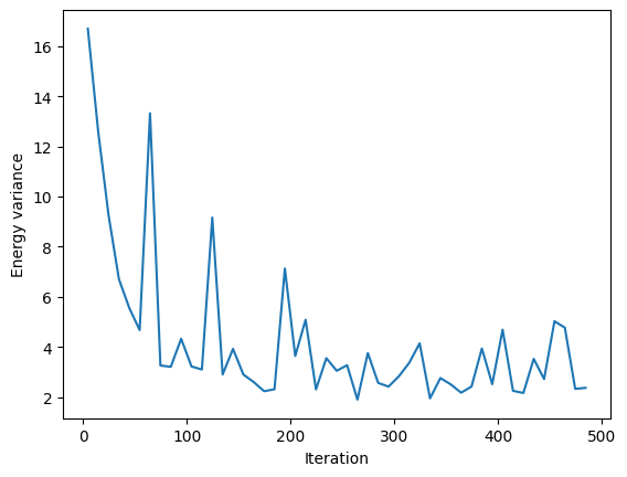
        VarE.plot(batch=10)
        plt.xlabel("Iteration")
        plt.ylabel("Energy variance")
        plt.show()

state.save("/tmp/neural_jastrow.eqx")

This state can also be symmetrized to achieve better accuracy

symm = C4v() @ SpinInverse()
state = qtx.state.Variational(
    model, param_file="/tmp/neural_jastrow.eqx", symm=symm, max_parallel=2048
)

sampler = qtx.sampler.SpinExchange(state, 1024, n_neighbor=[1, 2])
optimizer = qtx.optimizer.SR(state, H)

energy = qtx.utils.DataTracer()
VarE = qtx.utils.DataTracer()

for i in range(200):
    samples = sampler.sweep()
    step = optimizer.get_step(samples)
    state.update(step * 2e-3)

    energy.append(optimizer.energy)
    VarE.append(optimizer.VarE)

    if i % 10 == 0:
        clear_output()
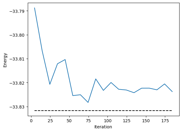
        energy.plot(batch=10, baseline=exact_energy)
        plt.xlabel("Iteration")
        plt.ylabel("Energy")
        plt.show()
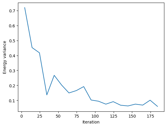
        VarE.plot(batch=10)
        plt.xlabel("Iteration")
        plt.ylabel("Energy variance")
        plt.show()

state.save("/tmp/neural_jastrow.eqx")

Then we can check its accuracy against the exact ground state.

dense = state.todense(full_symm).normalize()

E = dense @ H @ dense
print("Relative energy error:", abs(E - exact_energy) / abs(exact_energy))

fidelity = abs(dense @ exact_state) ** 2
print("Fidelity with exact ground state:", fidelity)

Relative energy error: 0.00017402258135205257
Fidelity with exact ground state: 0.99964914257028